How to Extract Data from a Spreadsheet using VLOOKUP, MATCH and INDEX

by Bob Flisser

When you need to find and extract a column of data from one table and place it in another, use the VLOOKUP function. This function works in any version of Excel in Windows and Mac, and also in Google Sheets. It allows you to find data in one table using some identifier it has in common with another table. The two tables can be on different sheets or even on different workbooks. There is also an HLOOKUP function, which does the same thing, but with data arranged horizontally, across rows.
The MATCH and INDEX functions are good to use when you’re concerned with the location of specific data, such as the column or row that contains a person’s name. 

Screencast

 

If you want to follow along with this tutorial using your own Excel file, you can do so. Or if you prefer, download the zip file included for this tutorial, which contains a sample workbook called vlookup example.xlsx.

Using VLOOKUP

When VLOOKUP finds the identifier that you specify in the source data, it can then find any cell in that row and return the information to you. Note that in the source data, the identifier must be in the first column of the table.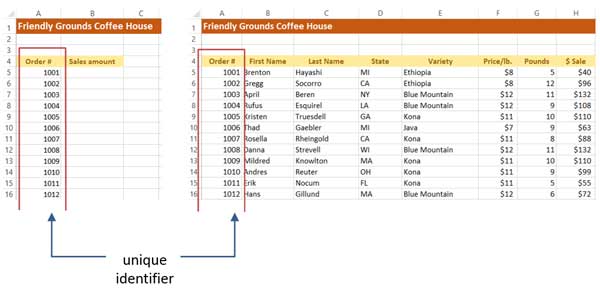

A unique identifier should be like a serial number, where no two are the same in the same table.

Syntax

The syntax of the VLOOKUP function is:
=VLOOKUP(lookup value, table range, column number, [true/false])


Here’s what these arguments mean:

• Lookup value. The cell that has the unique identifier.
• Table range. The range of cells that has the identifier in the first column, followed by the rest of the data in the other columns.
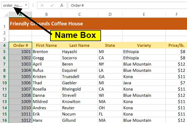
• Column number. The number of the column that has the data you’re looking for. Don’t get that confused with the column’s letter. In the above illustration, the states are in column 4.
• True/False. This argument is optional. True means that an approximate match is acceptable, and False means that only an exact match is acceptable.

We want to find sales amounts from the table in the illustration above, so we use these arguments:

Syntax of the VLOOKUP function

Define a Range Name to Create an Absolute Reference

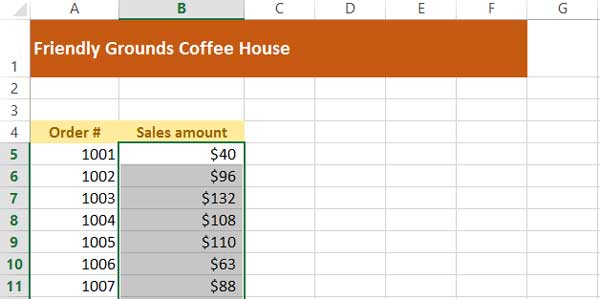
In Vlookup example.xlsx, look at the Sales Amounts worksheet. We’ll enter the formula in B5, then use the AutoFill feature to copy the formula down the sheet. That means the table range in the formula has to be an absolute reference. A good way to do that is to define a name for the table range.

Defining a Range Name in Excel

1. Before entering the formula, go to the source data worksheet.
2. Select all the cells from A4 (header for the Order # column) down through H203. A quick way of doing it is to click A4, then press Ctrl-Shift-End (Command-Shift-End on the Mac).
3. Click inside the Name Box above column A (the Name Box now displays A4).
4. Type data, then press Enter.
5. You can now use the name data in the formula instead of $A$4:$H$203.

The name box usually displays the current cell address. Click inside it and type a name to define a range.

Defining a Range name in Google Sheets

In Google Sheets, defining a name is a little different.

1. Click the first column header of your source data, then press Ctrl-Shift-Right Arrow (Command-Shift-Right Arrow on the Mac). That selects the row of column headers.
2. Press Ctrl-Shift-Down Arrow (Command-Shift-Down Arrow on the Mac). That selects the actual data.
3. Click the Data menu, then select Named and protected ranges.
4. In the Name and protected ranges box on the right, type data, then click Done.

Defining a range name in Google Sheets

Entering the Formula

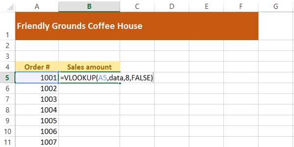
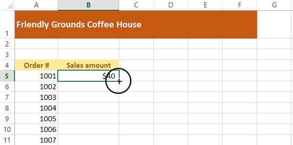
To enter the formula, go to the Sales Amounts worksheet and click in B5.
Enter the formula:
=VLOOKUP(A5,data,8,FALSE)
Press Enter.

Entering the VLOOKUP function

The result should be 40. To fill in the values down the column, click back on B5, if necessary. Put the mouse pointer on the AutoFill dot in the cell’s lower-right corner, so the mouse pointer becomes a cross hair.

When you place the mouse pointer on the dot in the lower-right corner of a cell, it becomes an AutoFill cross hair

Double-click to fill the values down the column.

Double-click the AutoFill cross hair to copy the formula down the column

If you want, you can run the VLOOKUP function in the next few columns to extract other fields, like last name or state.

Using MATCH

The MATCH function is doesn’t return the value of data to you; you provide the value that you’re looking for, and the function returns the position of that value. It’s like asking where is #135 Main Street, and getting the answer that it’s the 4^th building down the street.

Syntax

The syntax of the MATCH function is:
=MATCH(lookup value, table range, [match type])


The arguments are:

• Lookup value. The cell that has the unique identifier.
• Table range. The range of cells you’re searching.
• Match type. Optional. It’s how you specify how close of a match you want, as follows:

Next highest value	-1	Values must be in descending order.
Target value	0	Values can be in any order.
Next lowest value	1	Default type. Values must be in ascending order.

As with the VLOOKUP function, you’ll probably find the MATCH function easier to use if you apply a range name. Go to the Source Data sheet, select from B4 (column header for order #) to the bottom, click in the Name box above column A, and call it order_number. Note that the values are in ascending order.

A named range can be just one column, just one row, or even just one cell

Go to the Match tab of the worksheet. In B5, enter the MATCH function:
=MATCH(A5,order_number,1)

Entering the MATCH function

If you didn’t define a range name, you’d write the function as:
=MATCH(A5,'Source Data'!A5:A203,0)
Either way, you can see that this is in the 14th position (making it the 13^th order).

Result of the MATCH function

Using INDEX

The INDEX function is the opposite of the MATCH function and is similar to VLOOKUP. You tell the function what row and column of the data you want, and it tells you the value of what’s in the cell.

Advertisement

Syntax

The syntax of the INDEX function is:
=INDEX(data range, row number, [column number])
The arguments are:

• Data range. Just like the other two functions, this is the table of data.
• Row number. The row number of the data, which is not necessarily the row of the worksheet. If the table range starts on row 10 of the sheet, then that’s row #1.
• Column number. The column number of the data range. If the range starts on column E, that’s column #1.

Excel’s documentation will tell you that the column number argument is optional, but the row number is sort of optional, too. If the table range has only one row or one column, you don’t have to use the other argument.
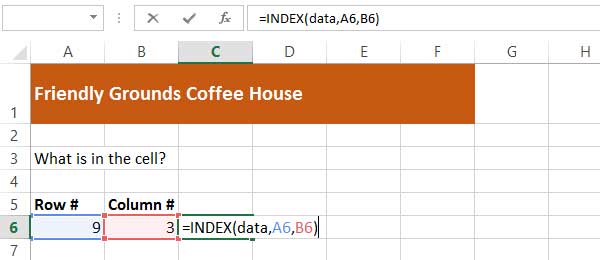
Go to the Index sheet of the workbook and click in C6. We first want to find what’s contained in row 9, column 3 of the table. In the formula, we’ll use the range name that we created earlier.
Enter the formula:
=INDEX(data,A6,B6)

entering the index function

It returns a customer’s last name: Strevell. Change the values of A6 and B6, and the result in C6 will show different results (note that many rows have the same states and product names).

Conclusion

The ability of a worksheet to look at another worksheet and extract data is a great tool. This way, you can have one sheet that contains all the data you need for many purposes, then extract what you need for specific instances.